class: center, middle, inverse, title-slide # Introduction to Spatial Data Analysis in R ## useR! 2022 ### Adithi R Upadhya, Meenakshi Kushwaha, and Pratyush Agrawal ### ILK Labs ### 20th June 2022 --- class:middle, center # Hi, Logistics alert ## [GitHub](https://github.com/adithirgis/user_2022_tutorial) ## [Slides](https://user2022tutorial.netlify.app/) ## [Read Me / Notes / Questions](https://docs.google.com/document/d/1OZUgLioKxihOVatHHnrFTNQn5ySHwKEfYhZGZuHxf9w/edit#heading=h.inqydmvlzlfh) ### We will start in 5 minutes. --- class:middle, center # A very brief intro to Map Projections  ??? We will start with a very brief intro to map projections. 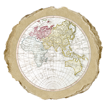Hopefully, it is just enough to help you get comfortable with basic concepts of spatial analysis in R --- # Map Projections .left-column[ 2-D representation of 3-D earth ] .right-column[  ] .footnote[https://gistbok.ucgis.org/bok-topics/map-projections] ??? 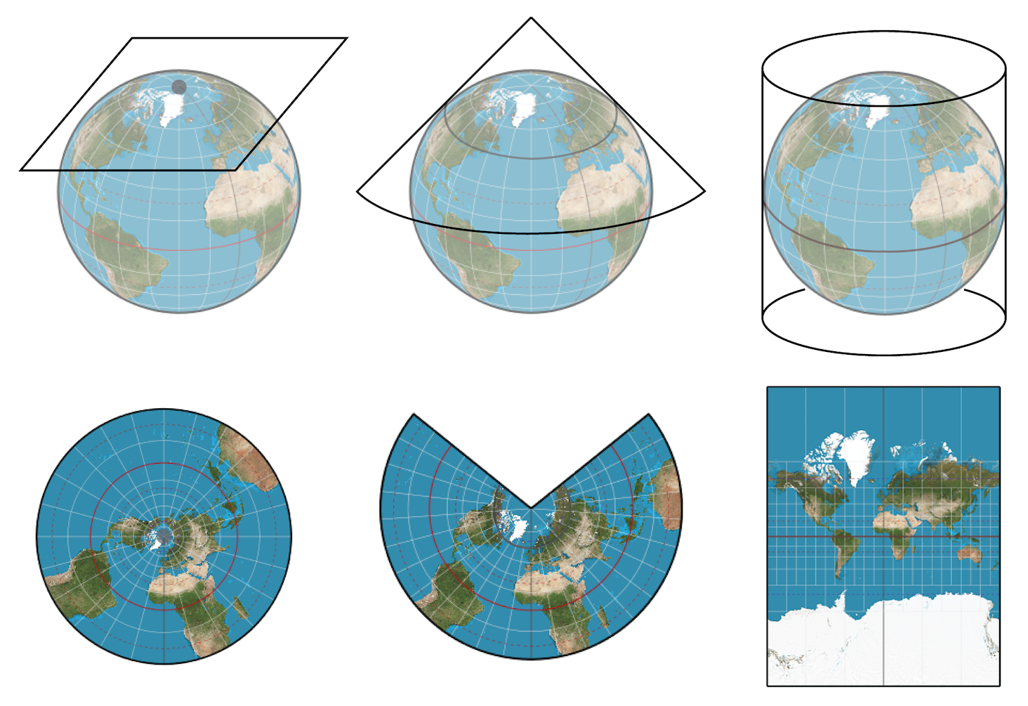Earth is a 3D object and when we are making a map we need to represent this in 2-D form i.e. on a flat surface. This is called MAP projections. As you can see in the figure here. There are several ways to do this. Think of keeping a paper either on the poles and project each point on that paper. Depending on how you project, your final map will be different. --- # Coordinate Reference Systems (CRS) Tell us how a map is related to real locations on earth ###Geographic vs Projected CRS  .footnote[Source:ESRI] ??? For example, a location of (130, 12) is not meaningful if you do know where the origin is and what the units are. Broadly, there are two categories of CRS. Geographic or unprojected, and it defines where the data is located on the earth’s surface as on the left. A projected CRS tells us how to draw on a 2-D flat surface, like on a paper map or a computer screen. A GCS is round, and so records locations in angular units (usually degrees). A PCS is flat, so it records locations in linear units (usually meters). --- ## CRS in R .pull-left[ - We need to know if the data is projected - which projection system is used - if not, you need to project it - use the correct system - most common projection is WGS84 - good for mapping global data - When data with different CRS are combined - need to transform them to a common CRS so they align with one another ] -- .pull-right[  #### Why so many CRS? - There are many different models of earth and so different algorithms for projection - Choice often based on minimum distortion for region of interest/parameter ] .footnote[https://www.esri.com/arcgis-blog/products/arcgis-pro/mapping/gcs_vs_pcs/] ??? Commonly used by organizations that provide GIS data for the entire globe or many countries. CRS used by Google Earth So, how to think about CRS in when you are doing your spatial analysis. . This is similar to making sure that units are the same when measuring volume or distances. It is usually impossible to preserve all characteristics at the same time in a map projection. This means that when you want to carry out your analysis, you need to use a projection that provides the best characteristics for your analyses. 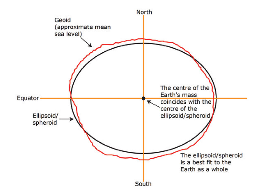--- # CRS in R .left-column[ ### Components of a CRS - projection - ellipsoid - defines general shape of earth - datum - defines origin ] .right-column[  ] .footnote[https://www.nceas.ucsb.edu/] ??? So, that sums up the theory part for this session. With this knowledge we hope that you'll have a good sense of handling projection of your data. 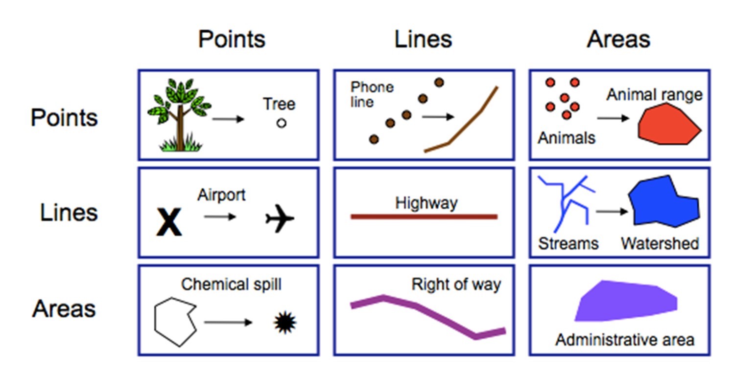--- background-image: url(img/bg_1.png) background-size:cover class: middle, center # Types of Spatial Data --- # Vector data .left-column[ - Points - Lines - Polygons ] .right-column[  ] .footnote[https://open.lib.umn.edu/mapping/chapter/4-design-and-symbolization/] --- # A different kind of data structure ### Vector data is stored in shapefiles *which is a set of files* .pull-left[ that store information about - location - shape - attributes of features file extensions - .shp, .shx, .dbf - .xml, .prj, .sbn, and .sbx - optional ] -- .pull-right[  ``` ] .footnote[Image: reddit] ??? In this format, information is distributed in multiple files. And as a beginner i have always done this. 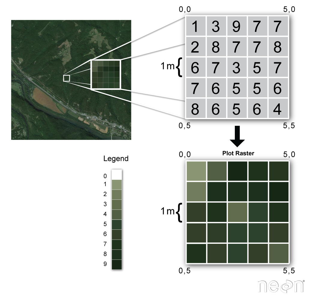--- # Raster data .left-column[ "gridded" data - saved in pixels file extensions - .jpeg, .tiff, .png ] .right-column[ <img src="img/raster_concept.png" width="80%" /> ] .footnote[Source: National Ecological Observatory Network (NEON)] ??? On the right, is a terresterial image, and we zoom in we see that each pixel repsents 1m2 and has a value. --- # Quiz Which of this is NOT a shape file - plants.csv - plants.shp - plants.dbf - plants.shx --- # Quiz Which of this is NOT a shape file - *plants.csv* - plants.shp - plants.dbf - plants.shx --- # Quiz Which of these is NOT a raster file - plants.xlsx - plants.png - plants.tiff - plants.jpeg --- # Quiz Which of these is NOT a raster file - *plants.xlsx* - plants.png - plants.tiff - plants.jpeg --- # Summary of Theory - Map Projections - Coordinate Reference Systems (CRS) - Types of spatial data - Vector - Raster --- class: middle, center background-image: url(img/bg2.png) background-position: center background-size: contain #R packages ###sf ###raster ###stars --- class:middle, center # 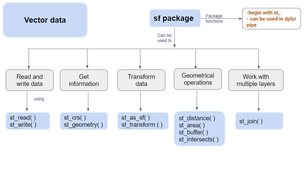sf  --- # [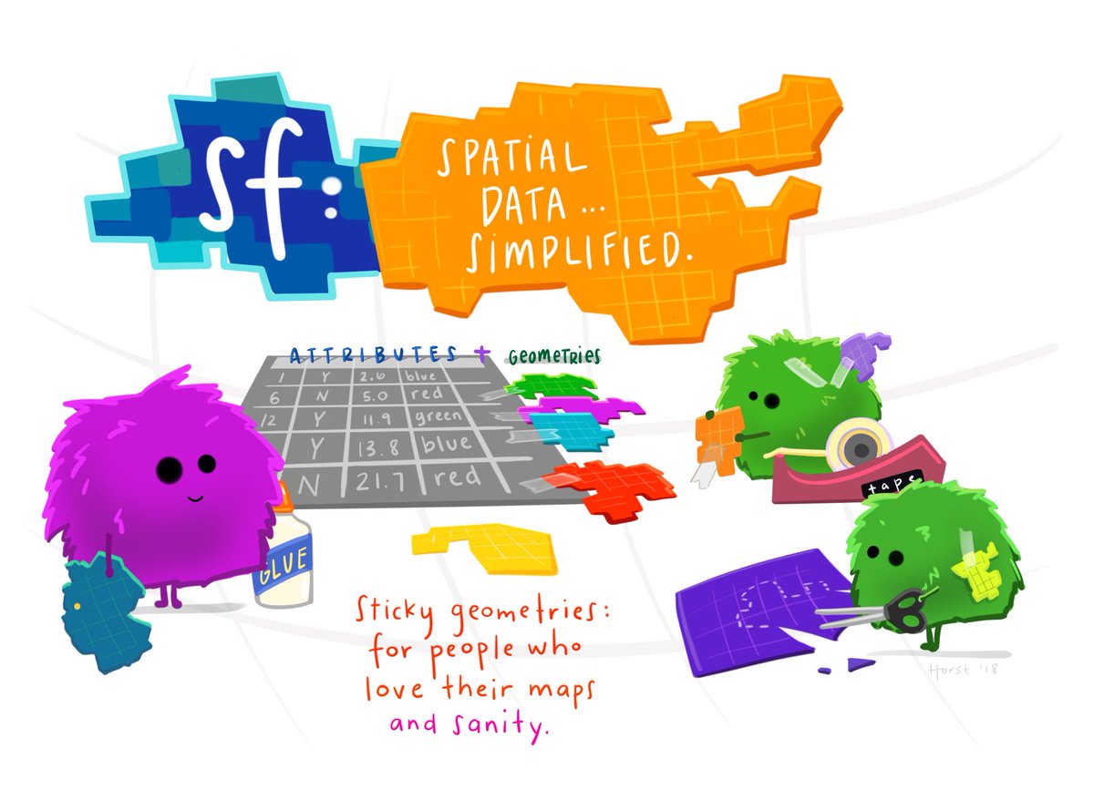sf package](https://cran.r-project.org/web/packages/sf/vignettes/sf1.html) Simple features are implemented using simple data structures (S3 classes, lists, matrix, vector). Similar to PostGIS, all functions and methods in sf that operate on spatial data are prefixed by st_. Typical use involves reading, manipulating and writing of sets of features, with attributes and geometries. <span role="img" aria-label="Three cute fuzzy monsters adding spatial geometries to an existing table of attributes using glue and tape, while one cuts out the spatial polygons. Title text reads “sf: spatial data...simplified.” and a caption at the bottom reads “sticky geometries: for people who love their maps and sanity."></span> ??? Use the sf package for simpler spatial data analysis with geometries that stick to attributes. As attributes are typically stored in `data.frame` objects (or the very similar `tbl_df`), we will also store feature geometries in a `data.frame` column. Since geometries are not single-valued, they are put in a `list-column`, a list of length equal to the number of records in the `data.frame`, with each list element holding the simple feature geometry of that feature. The three classes used to represent simple features are: `sf`, the table (data.frame) with feature attributes and feature geometries, which contains `sfc`, the list-column with the geometries for each feature (record), which is composed of `sfg`, the feature geometry of an individual simple feature. --- # Geometry types `POINT`: a single point `MULTIPOINT`: multiple points `LINESTRING`: sequence of two or more points connected by straight lines `MULTILINESTRING`: multiple lines `POLYGON`: a closed ring with zero or more interior holes `MULTIPOLYGON`: multiple polygons `GEOMETRYCOLLECTION`: any combination of the above types --- # Advantages of `sf` Is treated as a `data.frame` Can be used with a pipe operator Can be linked directly to the `GDAL`, `GEOS`, and `PROJ` libraries that provide the back end for reading spatial data, making geographic calculations, and handling coordinate reference systems --- # Load the libraries ```r library(sf) library(raster) library(tidyverse) library(stars) library(leaflet) library(ggplot2) library(ggspatial) ``` --- # Data used here - Vector data collected from lizards spread across urban Bangalore in 2022. - Raster data is temperature data downloaded from Google Earth Engine for the month of March 2022. --- # `st_as_sf` Convert foreign object to an `sf` object. ```r data <- read.csv("data/spotted.csv", sep = ",") prj4string <- "+proj=longlat +ellps=WGS84 +datum=WGS84 +no_defs" my_projection <- st_crs(prj4string) # Create sf object data_sf <- st_as_sf(data, coords = c("Longitude", "Latitude"), crs = my_projection) ``` The order of Longitude, Latitude, and the exact column names are important. PROJ4 formatted string list - https://proj.org/apps/proj.html. EPSG numeric code - https://proj.org/apps/proj.html. --- class:middle, center # Demo --- # Map ```r ggplot() + geom_sf(data = data_sf) + coord_sf() ``` --- class:middle, center # Demo --- # `st_is_valid` Checks whether a geometry is valid, or makes an invalid geometry valid. ```r st_is_valid(data_sf) ``` ``` ## [1] TRUE TRUE TRUE TRUE TRUE TRUE TRUE TRUE TRUE ``` --- # `st_write` and `st_read` Write simple features object to file or database. Read a simple features object. ```r st_write(data_sf, "data/spotted_sf.shp") # To save the XY or the coordinates use layer_options st_write(data_sf, "data/spotted_sf.shp", layer_options = "GEOMETRY=AS_XY") data_sf <- st_read("data/spotted_sf.shp") ``` --- # `st_point` Create simple feature from a numeric vector, matrix or list. ```r p1 <- st_point(c(2, 3)) p2 <- st_point(c(1, 4)) class(p1) ``` ``` ## [1] "XY" "POINT" "sfg" ``` --- # Geometry types `st_point` numeric vector (or one-row matrix) `st_multipoint` numeric matrix with points in row `st_linestring` numeric matrix with points in row `st_multilinestring` list with numeric matrices with points in rows `st_polygon` list with numeric matrices with points in rows `st_multipolygon` list of lists with numeric matrices `st_geometrycollection` list with (non-geometrycollection) simple feature objects --- # `st_crs` and `st_geometry_type` Retrieve coordinate reference system from `sf` object. Set or replace retrieve coordinate reference system from object. ```r st_crs(data_sf) ``` ``` ## Coordinate Reference System: ## User input: +proj=longlat +ellps=WGS84 +datum=WGS84 +no_defs ## wkt: ## GEOGCRS["unknown", ## DATUM["World Geodetic System 1984", ## ELLIPSOID["WGS 84",6378137,298.257223563, ## LENGTHUNIT["metre",1]], ## ID["EPSG",6326]], ## PRIMEM["Greenwich",0, ## ANGLEUNIT["degree",0.0174532925199433], ## ID["EPSG",8901]], ## CS[ellipsoidal,2], ## AXIS["longitude",east, ## ORDER[1], ## ANGLEUNIT["degree",0.0174532925199433, ## ID["EPSG",9122]]], ## AXIS["latitude",north, ## ORDER[2], ## ANGLEUNIT["degree",0.0174532925199433, ## ID["EPSG",9122]]]] ``` ```r st_geometry_type(data_sf) ``` ``` ## [1] POINT POINT POINT POINT POINT POINT POINT POINT POINT ## 18 Levels: GEOMETRY POINT LINESTRING POLYGON MULTIPOINT ... TRIANGLE ``` --- # `st_transform` Transform or convert coordinates of simple feature. ```r data_sf_projected <- st_transform(data_sf, 32643) ``` ??? 32643 is UTM projection with units m. --- class:middle, center # Demo --- class: inverse, center, middle background-image: url(https://www.valueresearchonline.com/content-assets/images/48497_measuring-the-world_02__w660__.gif) background-size: contain # Geometric measurements --- # `st_distance` Compute Euclidian or great circle distance between pairs of geometries; compute, the area or the length of a set of geometries. If the coordinate reference system of x was set, these functions return values with unit of measurement. ```r st_distance(data_sf_projected[c(1), ], data_sf_projected[c(5), ]) ``` ``` ## Units: [m] ## [,1] ## [1,] 17016.08 ``` --- # `st_area` Returns the area of a geometry, in the coordinate reference system used; in case x is in degrees longitude/latitude, `st_geod_area` is used for area calculation. Here we will use projected data to calculate area. --- class: inverse, center, middle background-image: url(https://cdn.dribbble.com/users/1002383/screenshots/4252960/v13.gif) background-size: contain # Geometric unary operations --- # `st_buffer` Buffer is determination of a zone around a geographic feature containing location that are within a specified distance of that feature. Computes a buffer around this geometry/each geometry. Returns a new geometry. Specify the radius of the buffer. ```r buf <- st_buffer(data_sf_projected, dist = 3000) ``` --- class:middle, center # Demo --- # More `st_boundary` returns the boundary of a geometry `st_centroid` gives the centroid of a geometry `st_reverse` reverses the nodes in a line `st_simplify` simplifies lines by removing vertices `st_triangulate` triangulates set of points (not constrained) `st_polygonize` creates polygon from lines that form a closed ring. In case of `st_polygonize`, x must be an object of class `LINESTRING` or `MULTILINESTRING`, or an sfc geometry list-column object containing these `st_segmentize` adds points to straight lines `st_union` combines several feature geometries into one, without unioning or resolving internal boundaries --- class: inverse, center, middle background-image: url(https://datavisdotblog.files.wordpress.com/2020/02/intersects-join-nx-30fps-33ms.gif) background-size: contain # Geometric binary predicates --- # `st_intersects` To find whether pairs of simple feature geometries intersect. Returns `TRUE` or `FALSE.` ```r st_intersects(data_sf_projected[1, ], data_sf_projected[2, ]) ``` ``` ## Sparse geometry binary predicate list of length 1, where the predicate ## was `intersects' ## 1: (empty) ``` --- class:middle, center # Demo --- # [More](http://postgis.net/workshops/postgis-intro/spatial_relationships.html) Geometric binary predicates on pairs of simple feature geometry sets. Return a sparse matrix with matching (`TRUE`) indexes, or a full logical matrix. `st_intersects` test whether Geometries/Geography spatially intersect `st_disjoint` returns `TRUE` if the Geometries do not spatially intersect - if they do not share any space together `st_touches` returns `TRUE` if the geometries have at least one point in common, but their interiors do not intersect `st_crosses` returns `TRUE` if the supplied geometries have some, but not all, interior points in common `st_within` returns TRUE if the first geometry is completely within the second geometry `st_contains` returns `TRUE` if the second geometry is completely contained by the first geometry `st_overlaps` returns `TRUE` if the Geometries share space, are of the same dimension, but are not completely contained by each other `st_equals` returns true if the given geometries represent the same geometry. Directionality is ignored `st_is_within_distance` returns `TRUE` if the geometries are within the specified distance (radius) of one another --- class:middle, center # Other operations --- # `st_join` ```r data_join <- read.csv("data/spotted_join.csv", sep = ",") # Create sf object data_join_sf <- st_as_sf(data_join, coords = c("Longitude", "Latitude"), crs = my_projection) # Join using predicate joined <- st_join(data_sf, data_join_sf, join = st_equals) ``` --- class:middle, center # Demo --- class:middle, center  ??? Summary of the vector data analysis till now. 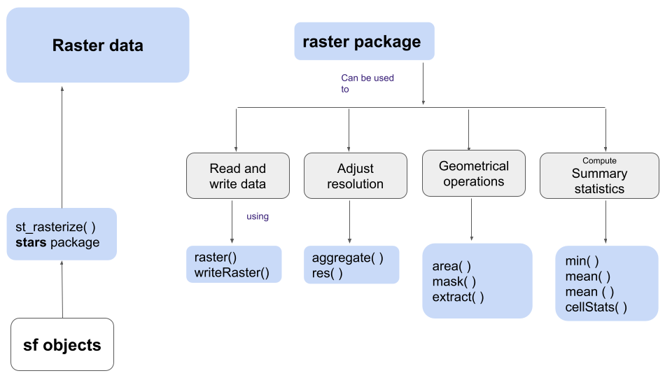--- class:middle, center # BREAK - 5 minutes --- class:middle, center # raster --- # Raster A `RasterLayer` can easily be created from scratch using the function raster. The default settings will create a global raster data structure with a longitude/latitude coordinate reference system and 1 by 1 degree cells. You can change these settings by providing additional arguments such as `xmn`, `nrow`, `ncol`, `res`, and/or `crs`, to the function. You can also change these parameters after creating the object. ```r temp <- raster("data/Ban_Temp_Mar2022.tif") y <- raster(ncol = 36, nrow = 18, xmn = -1000, xmx = 1000, ymn = -100, ymx = 900) ``` --- class:middle, center # Demo --- # Summary and Resolution `aggregate` - aggregates a Raster object to create a new RasterLayer or RasterBrick with a lower resolution (larger cells). ```r res(temp) ``` ``` ## [1] 0.1000005 0.1000005 ``` ```r summary(temp) ``` ``` ## Ban_Temp_Mar2022 ## Min. 297.7071 ## 1st Qu. 298.3609 ## Median 298.6290 ## 3rd Qu. 299.0802 ## Max. 300.2286 ## NA's 0.0000 ``` ```r temp_agg <- aggregate(temp, 2) res(temp_agg) ``` ``` ## [1] 0.2000009 0.2000009 ``` ```r res(y) ``` ``` ## [1] 55.55556 55.55556 ``` ```r summary(y) ``` ``` ## layer ## Min. NA ## 1st Qu. NA ## Median NA ## 3rd Qu. NA ## Max. NA ## NA's NA ``` --- # `projectRaster` To transform a `RasterLayer` to another coordinate reference system (projection) ```r # To transform temp_proj <- projectRaster(temp, crs = "+proj=utm +zone=43 +datum=WGS84") # To set the coordinate system projection(y) <- "+proj=utm +zone=48 +datum=WGS84" y ``` ``` ## class : RasterLayer ## dimensions : 18, 36, 648 (nrow, ncol, ncell) ## resolution : 55.55556, 55.55556 (x, y) ## extent : -1000, 1000, -100, 900 (xmin, xmax, ymin, ymax) ## crs : +proj=utm +zone=48 +datum=WGS84 +units=m +no_defs ``` ```r # To transform y_prof <- projectRaster(y, crs = "+proj=longlat +datum=WGS84 +no_defs") ``` --- class:middle, center # Demo --- # Summarizing functions Use `cellStats` to obtain a summary for all cells of a single raster object. ```r cellStats(temp, mean) ``` ``` ## [1] 298.7602 ``` --- # Raster algebra When used with a raster object as first argument, normal summary statistics functions such as `min`, `max`, and `mean` return a `RasterLayer` (usually for multiple layers). ```r r1 <- temp r2 <- r1 s <- stack(r1, r2) plot(max(s, na.rm = TRUE))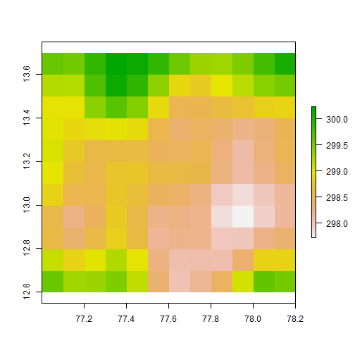 ``` <!-- --> --- # Extract Extract values from a `raster` object at the locations of spatial vector data ```r raster::extract(temp, data_sf) ``` ``` ## [1] 298.2247 298.2657 298.2442 298.2657 298.4747 298.2442 298.2442 298.6700 ## [9] 298.2657 ``` --- # Mask by buffer Mask values from a `raster` object at the locations of spatial vector data ```r data_sf_subset <- data_sf[1, ] data_sf_buffer <- st_buffer(data_sf_subset, dist = 5000) masked_raster <- mask(x = temp, mask = data_sf_buffer) ``` --- class:middle, center # Demo --- # Raster operation Returns a geographic subset of an object as specified by an Extent object (or object from which an extent object can be extracted/created) --- # Calculate area - Computes the approximate surface area of cells in an unprojected (longitude/latitude) `raster` object - returns all values or the values for a number of rows of a `raster` object. Values returned for a `RasterLayer` are a vector ```r sum(getValues(area(temp_proj))) ``` ``` ## [1] 21818160000 ``` --- class: middle, center # Demo --- # Rasterize using `stars` package ```r raster_data <- st_rasterize(data_sf) ``` --- class:middle, center # Demo --- # Vectorize using `stars` ```r tif <- read_stars("data/Ban_Temp_Mar2022.tif") summary(tif) class(tif) # Convert a foreign object to sf temp_sf <- st_as_sf(tif, as_points = TRUE) ``` --- class:middle, center # Demo ---  --- # Static Map ```r bangalore_boundary <- st_read("data/BBMP_Boundary.shp") bangalore_boundary <- st_transform(bangalore_boundary, crs = my_projection) ggplot() + geom_sf(data = bangalore_boundary, color = "green", size = 2, alpha = 0.1, fill = "green") + geom_sf(data = data_sf, color = "blue", size = 2) + theme_bw() + annotation_scale(location = "bl", width_hint = 0.5) + annotation_north_arrow(location = "bl", which_north = "true", pad_x = unit(0.75, "in"), pad_y = unit(0.5, "in"), style = north_arrow_fancy_orienteering) + coord_sf(xlim = c(77.4, 77.8), ylim = c(12.8, 13.2)) ``` --- class:middle, center # Demo --- # Interactive Map ```r leaflet(bangalore_boundary) %>% addTiles() %>% addPolygons(color = "green") %>% addCircles( data = data, lng = ~ Longitude, lat = ~ Latitude, radius = 20, weight = 20, fill = TRUE) ``` --- class:middle, center # Demo --- # Data Sources - [NaturalEarth](https://www.naturalearthdata.com/) supported by [`rnaturalearth`](https://cran.r-project.org/web/packages/rnaturalearth/README.html). - [OpenStreetMaps](https://www.openstreetmap.org/) supported by [`osmdata`](https://cran.r-project.org/web/packages/osmdata/index.html). - [ETOPO5](https://www.ngdc.noaa.gov/mgg/global/etopo5.HTML) elevation data. - [Movebank](https://www.movebank.org/cms/movebank-main) animal movement data. - [EuroStat](https://ec.europa.eu/eurostat) provides European Statistics and Indicators. - [Global Human Settlement Layer](https://ghsl.jrc.ec.europa.eu/) provides population data and other similar datasets. - [USGS Global Island Explorer](https://rmgsc.cr.usgs.gov/gie/) island datasets. - [spData](https://cran.r-project.org/web/packages/spData/spData.pdf) diverse spatial datasets for demonstrating and teaching spatial data analysis. --- # Sometimes.. - Making maps in R is not always easy. - It is slow. - Map transformations can be a problem. - Adding annotations can be tedious. --- # Resources used https://bookdown.org/nicohahn/making_maps_with_r5/docs/ggplot2.html#using-ggplot2-to-create-maps https://www.youtube.com/watch?v=qbrnzSRPyb0 https://geocompr.robinlovelace.net/spatial-class.html https://github.com/statnmap/user2020_rspatial_tutorial https://www.jessesadler.com/post/simple-feature-objects/ https://heima.hafro.is/~einarhj/spatialr/pre_sf.html https://cran.r-project.org/web/packages/sf/vignettes/sf1.html https://mgimond.github.io/Spatial/raster-operations-in-r.html#computing-cumulative-distances https://r-spatial.github.io/stars/ Images from [rawpixel](https://www.rawpixel.com/) --- # THANK YOU - [Adithi R Upadhya](https://adithirugis.rbind.io/) - [Meenakshi Kushwaha](https://meenakshi.rbind.io/) - [Pratyush Agrawal](https://twitter.com/Pratyushagraw97) --- class:middle, center # Excersise - 20 minutes --- class:middle, center # Questions?